Lazy reader’s guide: skip to the pretty pictures, skim the conclusions section, ignore the rest.
Background
I think a lot about eigenvalue and singular value decompositions. I won’t get into it right now, but I have been quoted in the past as saying that singular values are eigenvalues for grownups. But today we need to go back to gradeschool to talk about singular values for babies: eigenvalues.
In R, most of your linear algebra is handled by the BLAS and LAPACK libraries. The BLAS handles really basic vector and matrix operations, while LAPACK has all the fun stuff like factorizations, including eigenvalues. This bit is important but has been written about ad infinitum, so I’ll keep it brief: use good BLAS. R ships with the Reference BLAS, which are slow. If you don’t know what any of this means, the easiest way forward is to just download Microsoft R Open (formerly from Revolution Analytics). It’s basically R compiled with Intel compilers and shipped with MKL (good BLAS, and more actually).
There are about a million ways to compute eigenvalues in LAPACK, but if your data looks like the way we store matrices in R, there are two significant ones: relatively robust representations (RRR) and divide and conquer (D&C). If you search around, you will find people generally say that
- RRR is faster than D&C
- RRR uses less RAM than D&C
But I couldn’t really find much more detail than that. I’ve been doing some experiments of my own with computing eigenvalues in the band package, which is a new framework for handling banded matrices in R. In the course of my experiments, I made a wrapper for the D&C method, and ended up comparing it against R. My implementation was faster, by a margin that made me raise an eyebrow. Eventually I figured out that R uses the RRR method; but this seemed to run counter to the internet wisdom that D&C is slower.
The great thing about doing computational work is that you don’t have to accept anybody else’s bullshit. We can test this, and I don’t need a team of researchers or grant money or IRB signatures or anything. We just need a free afternoon and a little elbow grease.
The Benchmark
The quick summary is that we’ll be measuring RRR versus D&C wall clock run times with 5 replications with the following variations:
- 9 different problem sizes (“n”), namely 25, 50, 100, 250, 500, 1000, 2000, 4000, and 8000.
- 4 different BLAS libraries: Reference, Atlas, OpenBLAS, and MKL.
Hardware is a 4 core Intel Core i5-2500K CPU @ 3.30GHz. Additional software is as follows:
- R 3.1.1
- gcc 6.2.0-5
- Microsoft R Open 3.3.1 and Intel MKL
- Whatever versions of Reference, Atlas, and OpenBLAS that are in Ubuntu 16.10 at the time of writing.
Reference and Atlas timings are with one core; OpenBLAS and MKL are with 4.
Results
Displaying all of this is kind of difficult, but ggplot2 certainly does make the process less painful. And I’ve never claimed to be a vis expert; so I’d better not see a bunch of vis hipsters posting sassy bullshit on twitter over my plots.
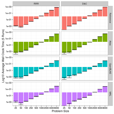
There are several things that are striking in this first plot:
- MKL is only slightly faster than OpenBLAS; both are much faster than Atlas and Reference BLAS (old news).
- There’s very little variability in the run times, particularly for the larger problem sizes.
- We still haven’t really answered our original question.
To better address the RRR vs D&C bit, let’s focus in only on the two largest problem sizes:
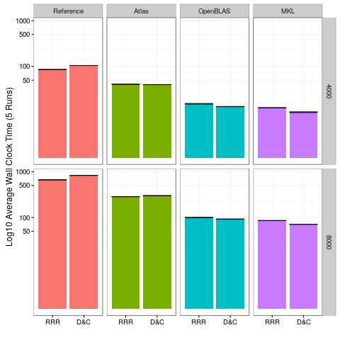
For both the 4000 and 8000 problem sizes, it’s pretty obvious that D&C is faster with OpenBLAS and MKL, and slower with Reference and Atlas. So it feels like we have our answer. But feels can be deceiving.
Now after seeing this second plot, I was just about ready to call it a day. But then I started thinking; the two benchmarks where D&C consistently won were OpenBLAS and MKL, which each were using 4 cores. By contrast, Atlas and the Reference BLAS (the two where D&C lost) were strictly serial. What if these didn’t actually have faster D&C implementations, but that D&C was simply more scalable?
Turns out my hunch was correct:
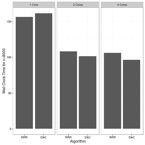
This run was with OpenBLAS only; we would almost certainly see the same results with MKL. But I also use this machine to watch Netflix, so I’m gonna stop heating up my house with benchmarks and go watch Star Trek.
So there. We settled it…
But Wait! There’s More!
We still haven’t looked at the memory allocation issue. This is actually much easier than you might expect if you’ve never worked with LAPACK before. The reason is, LAPACK was originally written in Fortran 77 — a language that does not support dynamic memory allocation. So any time a function (subroutine in Fortran) needed some local workspace, then you had to allocate it for that function. So all LAPACK functions are very up front in the documentation about allocation sizes. They even have a cute way of telling you the allocation requirements at run time.
Anyway, D&C uses the dsyevd() function, and RRR dsyevr() (links are to original Fortran source code). You can skim the source to see if I’m lying to you, or take my word for it that the memory requirements are:
library(memuse)

dnc = function(n) mu(1+6*n + 2*n*n)*8 + mu(3 + 5*n)*4
rrr = function(n) mu(26*n)*8 + mu(10*n)*4
Now, if you’re willing to destroy the input data, then this calculation is a little unfair to D&C; they get much closer in terms of the total amount of memory required to allocate to perform the calculation. But in R, we can’t destroy the input data, so for any R bindings, that is ultimately irrelevant. Also, the RRR version is a lower bound of the additional memory requirements. I went to the trouble to check what it’s actually using on my machine, and it’s never more than 2x the lower bound. You’re about to see why this factor of 2 is irrelevant.
Here are some figures for our n=8000 problem size:
n = 8000

# Size of an 8000x8000 matrix
howbig(n, n)
## 488.281 MiB

# Extra memory use for D&C method
dnc(n)
## 977.081 MiB

# Extra memory use for RRR method
rrr(n)
## 1.892 MiB
Pretty striking. If we had a problem size that pushed the RAM limits of most modern workstations, it doesn’t get any better:
n = 46340

# Size of a 46340x46340 matrix
howbig(n, n)
## 15.999 GiB

# Extra memory use for D&C method
dnc(n)
## 32.002 GiB

# Extra memory use for RRR method
rrr(n)
## 10.960 MiB
Conclusions
- If you don’t know how to manage the BLAS that you’re using, for god’s sake just use the Revolution/Microsoft distribution of R.
- RRR has better runtime performance than D&C in serial, and worse in parallel.
- D&C gobbles up RAM at an astounding rate.
- People who say that the D&C method is slower are not quite right, or at least not completely right.
- People who say that the D&C method uses more RAM are underselling their case.
- It would be really interesting to see how this scales with accelerator cards, like GPU’s and Intel MIC.
Data and R Scripts
Here’s the data:
And here’s the benchmarking script. I gave it the very descriptive name x.r:
type = commandArgs(trailingOnly=TRUE)

library(band)
library(coop)

data = function(n)
{
  x = rnorm(n*n)
  dim(x) = c(n, n)
  covar(x)
}


nreps = 5

N = c(25, 50, 100, (2^(0:5))*250)

rowlen = length(N)*nreps
df = data.frame(numeric(rowlen), character(rowlen), numeric(rowlen), numeric(rowlen), stringsAsFactors=FALSE)
colnames(df) = c("n", "type", "RRR", "D&C")

row = 1L
for (n in N){
  x = data(n)

  for (rep in 1:nreps){
    eigen_r = system.time(eigen(x))[3]
    eigen_me = system.time(eig(x))[3]
    df[row, ] = c(n, type, eigen_r, eigen_me)
    row = row+1L
  }
}
Invoke this via Rscript x.r NameOfBLASLib. So for example, if we were running with OpenBLAS, we’d use:
Rscript x.r OpenBLAS
Now unfortunately, this naming scheme doesn’t actually set the BLAS library. It’s only for plotting later. I ran this on an Ubuntu machine, where changing BLAS is trivial. Simply run:
sudo update-alternatives --config libblas.so.3
from the command line and choose the one you want. On other systems you have to swap things out manually, or possibly even rebuild R.
As for the plots, if you read in the eig_bench.csv data above to the R object df, then this is straightforward:
library(reshape2)
library(plyr)
dfm = melt(df, id.vars=c("n", "type"))

se = ddply(dfm, c("n", "type", "variable"), summarise, mean=mean(value), se=sd(value)/sqrt(length(value)))
se = transform(se, lower=mean-se, upper=mean+se)

library(ggplot2)
library(scales)
ggplot(se, aes(n, mean, fill=type)) +
  theme_bw() +
  geom_bar(stat="identity") +
  guides(fill=FALSE) +
  facet_grid(type ~ variable) +
  xlab("Problem Size") +
  ylab("Log10 Average Wall Clock Time (5 Runs)") +
  scale_y_log10() +
  geom_errorbar(data=se, position=position_dodge(0.9), aes(ymin=lower, ymax=upper))
The other two plots are pretty obvious variations of this; subset for the second, use the other dataset for the third. Consider it an exercise.
A Note About Benchmarking
Choosing sizes for benchmarking is important. The problem sizes I chose aren’t arbitrary. Well…they’re kind of arbitrary, but not completely.
When you’re benchmarking, it’s very important to pick the right size of data. If you’re only interested in microsecond performance (say you need to execute something millions+ times per second), for one, stop using R immediately, you’ve made a terrible mistake. And two, you probably don’t care about large problem sizes. The same is true in reverse. If you only care about large problems, then who cares if it’s “slow” on small ones; you’re probably only thinking about something executing once.
So what if you care about both? A lot of people get this wrong for some reason, but the short version is that you should look at lots of varying problem sizes. In particular, you should make sure your data no longer comfortably fits in cache. If you haven’t measured the performance of your implementation at, say, 2x the size of your largest cache, then whatever claims you have about performance are complete bullshit. Period.
Fortunately, in R we can look up cache sizes very easily with the memuse package. This is the result from my machine (the one I ran the benchmarks on):
memuse::Sys.cachesize()
## L1I:   32.000 KiB
## L1D:   32.000 KiB
## L2:   256.000 KiB
## L3:     6.000 MiB
My biggest cache is L3, at 6 megs. Some server hardware even has L4 cache these days! Anyway, always make sure that your data doesn’t fit in cache, because this can hide terrible performance patterns.
There’s a very simple test we can do to prove this. We’ll use compiled code by way of Rcpp, because I need to have more control over the demonstration than I can get with pure R code (R functions have a lot of overhead and variability that get in the way, but this is still valid for pure R code). We’re going to create a function that takes an integer input n and output an nxn matrix of all 1’s. And we’ll do this in two ways, first by iterating over the rows then columns of the matrix, and second by iterating columns first then rows. We’ll name them, oh I don’t know, bad() and good() respectively, for no particular reason. Also for no particular reason, you should know that matrices in R are column-major.
Anyway, here they are:
#include <Rcpp.h>

// [[Rcpp::export]]
Rcpp::NumericMatrix bad(const int n)
{
  Rcpp::NumericMatrix x(n, n);

  for (int i=0; i<n; i++)
    for (int j=0; j<n; j++)
      x(i, j) = 1.;

  return x;
}

// [[Rcpp::export]]
Rcpp::NumericMatrix good(const int n)
{
  Rcpp::NumericMatrix x(n, n);

  for (int j=0; j<n; j++)
    for (int i=0; i<n; i++)
      x(i, j) = 1.;

  return x;
}
Save them as cache_eg.cpp and run the following in R to build them:
library(Rcpp)
library(microbenchmark)
library(memuse)

sourceCpp("cache_eg.cpp")
We can test on a small matrix:
n = 100L
howbig(n, n)
## 78.125 KiB

mb = microbenchmark(bad(n), good(n))
boxplot(mb)
And these look pretty close; maybe we shouldn’t have called one of them bad() after all?
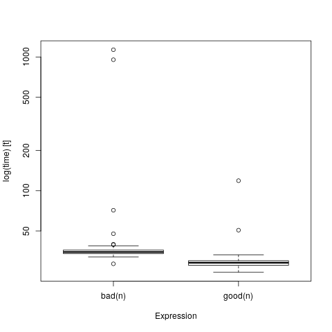
Let’s try a larger data size…
n = 4000L
howbig(n, n)
## 122.070 MiB

mb = microbenchmark(bad(n), good(n))
boxplot(mb)
HOLY SHIT WHAT HAPPENED?!
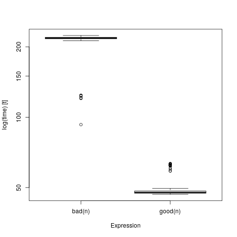
This problem was deliberately cooked up to make this kind of comparison; we could actually make it worse by adding parallelism, but generally it won’t look this bad even if you screw your data accesses up. But if you’re only ever comparing two functions on teensy tiny data, you can not possibly know how well it will perform on datasets that don’t fit in cache.
To better understand why this is so important, here’s a fun little interactive visualization showing the relative speeds in fetching data from RAM versus cache. You may also be interested in some of my older posts Cache Rules Everything Around Me and Advanced R Profiling with pbdPAPI.